Examples gallery¶

Runnable scripts that render the figures in the docs and README. They are not part of the installed package (only src/cpomdp ships in the wheel) — they import plotting libraries the core does not depend on. The examples are not subject to the same level of precision as the rest of cpomdp. They are here as showcases. The numbers in them are not citable facts.

Get the plotting deps with the examples extra:

pip install "cpomdp[examples]"        # then: python examples/<script>.py

…or, from a source checkout, with uv (no install needed):

uv run --extra examples python examples/<script>.py

Each script writes its asset into ../docs/assets/ and takes an optional output path as argv[1].

Flagship — instrumental epistemics: the beacon resolves food location¶

bacillus_uncertain_food.py · v0.4 · ADR-013

Expected Free Energy decomposes into an epistemic (information-seeking) value and a pragmatic/instrumental (goal-seeking) value. Epistemic value is genuinely instrumental — not merely curious — when the uncertainty it resolves is decision-relevant: the discrete T-Maze task (Friston et al. 2015, "Active inference and epistemic value") is the canonical case, where visiting a cue resolves which arm holds the reward, changing the subsequent action. The v0.3 demo below ties the beacon's epistemic value to the agent's own position — salience without an instrumental payoff, since knowing your own position more precisely doesn't change which action is later correct. This flagship promotes the food's position to an explicit latent the agent does not know a priori, and rewires the beacon to resolve that instead — now the resolved uncertainty changes where the agent then heads, the property the v0.3 demo's epistemic value lacked. The whole change is one rewiring, the beacon mechanic itself untouched:

# v0.3: the state is the agent's position, and the one channel reads it. The noise
# that channel carries is keyed on that SAME position — self-revealing.
observation_matrix = I                      # C: o = agent_xy            (2x2)
noise_fn(x, p) = beacon_noise(x, p)   # R(x): keyed on the channel's own block

# v0.4: the state gains the food's position as a latent, and a second pair of rows
# reads the DISPLACEMENT to it. The noise is still keyed on the agent's own
# position block, exactly as before.
observation_matrix = [[I, 0],               # C: rows 1-2  o = agent_xy   (4x4)
                [-I, I]]              #    rows 3-4  o = food_xy − agent_xy
noise_fn(x, p) = beacon_noise(x[:2], p)  # R(x): still keyed on agent_xy only

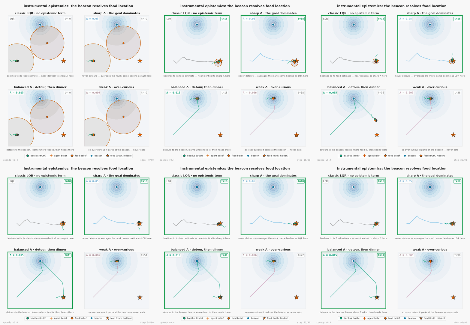
Same four-regime structure as the v0.3 demo, same single real knob (the goal precision Λ): classic LQR and a sharp Λ both beeline toward the current food estimate and never detour — with LQR's effort cost set to ≈0 to match the EFE selection (which has none), the two are the same controller here, ADR-003's fixed-sensor collapse (EFE reduces to LQR) made visible; a balanced Λ detours to the beacon, learns where food really is, then heads there with confidence; a weak Λ is so over-curious it parks at the beacon and never eats. Each panel carries its own t= step counter and border, which turn green and freeze the moment that regime first settles near the food, so the GIF shows directly when each one gets there, not just whether.

That border cue is also what makes the detour's actual cost legible: the balanced regime is not the fastest. The two beeliners — classic LQR and sharp Λ=0.05 — settle soonest, together at step 18 of 90 on near-identical shortest paths (9.6 and 9.9 units travelled); balanced (Λ=0.015) is the slowest of the regimes that arrive at all (step 41) and travels the farthest (≈13.8 units), because it deliberately detours. What that detour buys is precision, not speed: once settled, balanced's belief about the food's location is roughly 7x tighter than the beeliners' (final covariance trace ≈0.004 vs ≈0.029) and its final position error is close to four times smaller (0.04 vs 0.15 and 0.18). It is an explore/exploit trade — time and distance traded for confidence — not a regime that wins on every axis.

The simulation is checked, not just rendered: every agent's filter is run through both inference backends, and --scan checks the native KalmanBackend and the v0.4 FFG ChainBackend agree to atol=1e-7.

Four bacilli learning where the food is, under different goal precisions Λ

bacillus_uncertain_food.py --scan prints the regime metrics and the Kalman-vs-ChainBackend agreement check without rendering.

Forney-style Factor Graph (FFG) examples — branching factor graphs¶

The v0.4 examples that need a branching model rather than a chain live in their own sub-gallery — the dissociation demo (a branch-coupled R(x) sensor that can't be flattened to a Kalman filter), the coupling-graph figure, and a chemotaxis-network figure. See ffg/README.md.

R(x) and a long enough H bring curiosity back to a linear-Gaussian agent¶

crossover_horizon_figure.py

Under a fixed linear-Gaussian sensor the epistemic term of expected free energy is a constant across policies. It cannot change any decision. The agent reduces to LQR, the collapse efe_collapse_figure.py draws. A state-dependent R(x) breaks that: the action reaches the noise, so curiosity becomes possible again. Possible is not the same as decisive.

An open plane. The agent wants to be at a goal it cannot locate. Its prior says the goal is over to the right. It is not. A beacon well off that line is the only thing that can tell it where the goal really is. Walking there costs ground.

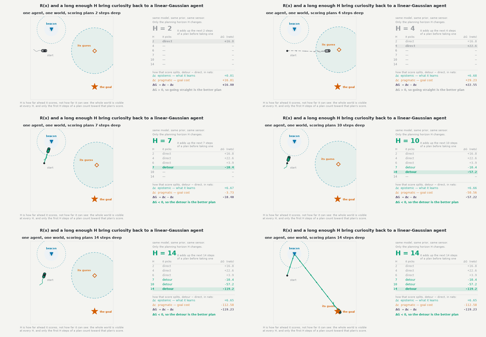
The animation runs the same world once per planning horizon, and the ladder on the right fills in as it goes. At a short horizon the agent walks straight to the spot it already believed in and settles there. It never checks. Somewhere in the sweep it stops doing that: it walks away from where it thinks the goal is, reads the beacon, finds out it was wrong, and then goes to the real one. Nothing changed but H. Same model, same prior, same sensor, same two candidate plans, same objective.

One agent run once per planning horizon: at short horizons it settles where its prior said, and past a crossing it detours to the beacon, learns where the goal really is, and goes there

Reading the numbers beside the animation¶

Expected free energy splits in two, G = c − ε:

c, the pragmatic term. How far the observations a plan expects to get sit from the ones the agent prefers. Here: how far from the goal it ends up.
ε, the epistemic term. How much the agent expects that plan to teach it. Here: how much sharper its belief about where the goal is will be.

Lower G wins, so a plan is worth taking when what it teaches outweighs what it costs.

Every number shown is a difference between the two candidate plans, detour minus direct, in nats:

quantity	what it is
`Δε = ε(detour) − ε(direct)`	the extra information the detour buys
`Δc = c(detour) − c(direct)`	the extra goal cost it pays for it
`ΔG = Δc − Δε = G(detour) − G(direct)`	which plan wins

The difference is the whole decision: whatever the two plans have in common cancels out of it, so the absolute G of either one tells you nothing about which gets picked. ΔG above zero and the agent goes straight. Below zero and it detours. That is also why the ladder swings from +16.8 to −119.2. Neither plan "has" that score. It is how far apart they are, and the gap widens as the horizon gives the detour more steps to collect on what it learned.

What "planning horizon" means here¶

H is how many steps of a plan the agent adds up when it scores that plan. Not how far it can see. Perception does not change with H at all: the world is fully visible throughout, and the beacon is exactly as informative to an H = 2 agent standing on it as to an H = 14 one. What H changes is how much of a plan's consequence is inside the window when the agent commits to its next single step.

Two steps cannot reach the beacon. The information it would buy falls outside the window entirely and never reaches the balance sheet: Δε there is under 0.01 nats, essentially nothing. By H = 7 the sensing step is inside the window, and so are the steps that cash in on it.

Why the horizon decides it¶

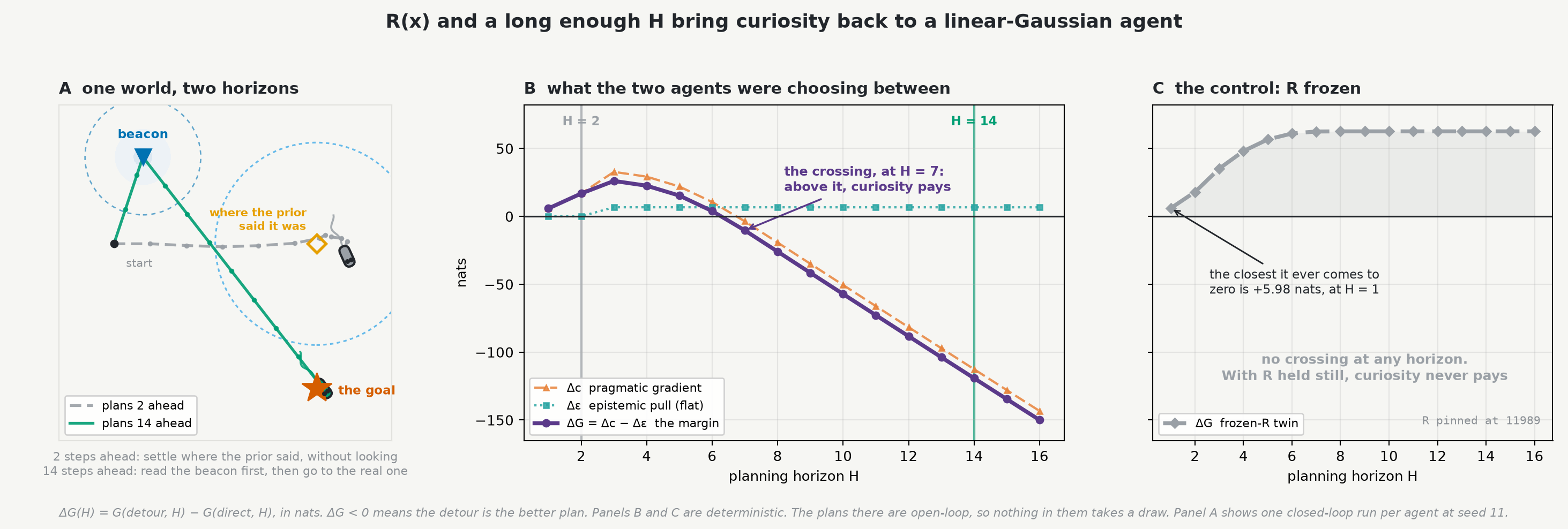
The epistemic pull is flat. Sensing once is worth what sensing once is worth, so Δε does not grow with the horizon. What moves is Δc. After the detour the sharpened goal belief lowers the expected goal cost on every remaining step, and that saving accumulates until it covers the one-off cost of walking off course. So the direct plan's advantage decays under a constant pull, and ΔG crosses zero exactly once.

The right-hand panel below is the control. A beacon-and-goal task on a plane looks like the discrete cue tasks people already know, so the whole sweep is re-run with R frozen at a constant, everything else identical. Curiosity then never pays at any horizon. What freezing R zeroes is Δε, not ε. With a fixed noise the covariance recursion stops consulting the action, so both plans carry the identical covariance sequence and whatever either one learns cancels out of the difference. Each plan's own ε is still nonzero and still grows with H. Action-invariance is the collapse, not absence. It takes R(x) and the horizon.

The margin between the two plans against the planning horizon, crossing zero once, beside a frozen-R control that never crosses

--check prints the sweep and asserts what the figures claim, with no plotting deps. Everything asserted is open-loop, so none of it takes a seed. The animated runs take one, named in the caption. Where the crossing lands belongs to these particular numbers. The shape carries over. The integer does not.

This is not the registered `H*`¶

The library's H* is also 7, and the two have nothing to do with each other. That one is an exhaustive |A|^H search over a declared, versioned action set on the two-node coupled cue tree, with the epistemic term restricted to the context node, and it carries a completeness certificate. Its Δε at H = 1 is 1.72 nats.

This demo scores two named plans on a flat four-dimensional chain, takes the epistemic term over the whole state, and searches nothing at all. Its Δε is 6.67 nats. The two integers coincide. Nothing follows from that, and neither number should be quoted as the other.

The difference is what each one is entitled to claim. An exhaustive enumeration over a declared finite set decides that no policy in the set flips, which is why the corridor result carries PROVED and a completeness certificate. A two-policy contrast decides nothing about the argmin: the best plan at any horizon could be a third one neither of these. So the crossing drawn here is an exact fact about a detour and a direct route, and the plane is where the mechanism is legible rather than where it is established. The corridor is the proof, in ffg/crossover.py and warrant_numbers.md, and it answers a question left open by arXiv:2607.20306: that paper gets the epistemic term to stop being constant, and stopping being constant is not yet changing a decision.