Forney-style Factor Graph (FFG) examples — branching factor graphs
The v0.4 examples that need a branching model, not a chain. A chain is the one shape a Kalman filter already is; these are the shapes it isn't. Part of the examples gallery.
Get the plotting deps with the examples extra:
…or from a source checkout, with uv:
Each script writes its asset into ../../docs/assets/ and takes an
optional output path as argv[1].
A branch-coupled R(x) can't be flattened
epistemic_dissociation_figure.py · v0.4 · ADR-019, ADR-020, ADR-021
Why build an FFG instead of a flat Kalman/EFE loop? Because some models a flat loop can't
run. Give a node a state-dependent sensor R(x), couple it to a hidden context, then ask
cpomdp to flatten the model to a plain Kalman filter — it won't. A flat Kalman linearises the
noise at the prior mean μ⁻; the factor graph linearises at the coupling-resolved μ⁺; the
coupling makes those differ, so no fixed linear-Gaussian model reproduces R(μ⁺). You get
IncompatibleLinearizationError. The fixed-sensor version flattens fine (μ⁻ = μ⁺), so the
clash is R(x) plus a coupling, not the branching. That inexpressibility is the reason to
reach for the FFG here; the A-vs-B behaviour below is what it buys.
Two agents run the same maze, the same goal, and the same FfgEfeSelector. One line differs
— the cue sensor:
cue = (CallableGaussianObservation(observation_matrix, cue_noise, params)  # B: R(x), alive
       if epistemic_alive
       else GaussianObservation(observation_matrix,
                                observation_noise=fixed_noise))     # A: fixed, dead
B's R(x) is sharp only at the cue, so R(μ⁺) moves with the action (the dual effect,
ADR-019). Its epistemic term is live: B detours to read the cue, resolves the hidden
CONTEXT through the branch, and crosses to the right arm. A's fixed sensor gives a constant
epistemic term (Koudahl–Kouw–de Vries 2021, ADR-003), so it falls back to the LQR choice and
stays at the wrong arm. Same maze, same goal; B's final belief about which arm pays is ≈11x
tighter. A control statement, not biology (ADR-020).
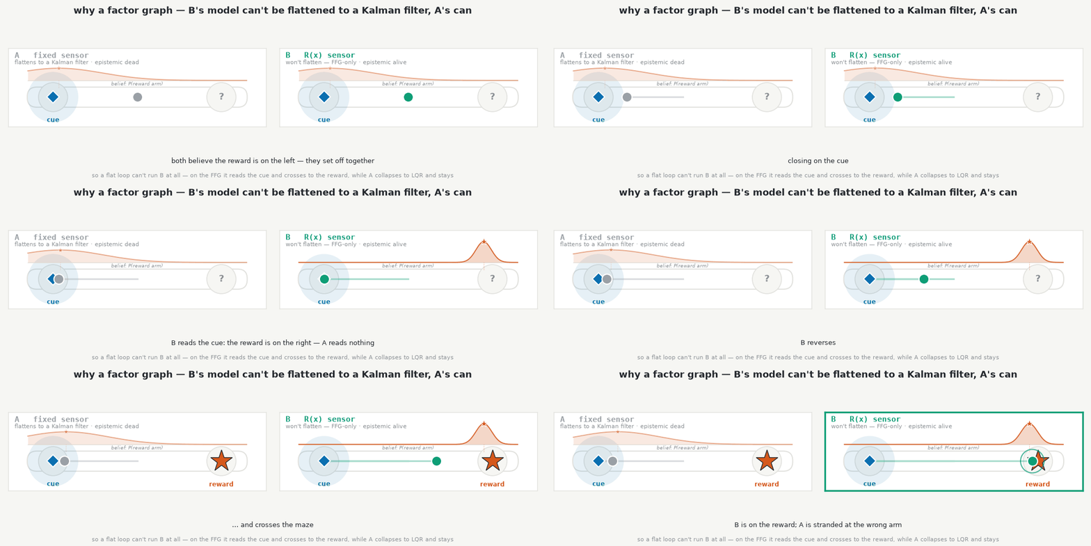
epistemic_dissociation_figure.py --check asserts the four results — the raised error, B's
resolved latent, the dual effect (B's epistemic moves, A's is flat), and the confound-free
horizon-1 ordering (epistemic pull < pragmatic gradient) — without rendering.
Declare the structure, skip the joint
coupling_graph_figure.py · v0.4 · ADR-012, ADR-014
The factor graph earns its keep the moment the model branches: a hidden root r seen only
through a hub h that fans out to two observed leaves, a degree no chain can hold. The
figure puts CouplingGraph.infer (name the edges, call once) beside the 4×4 joint precision
a normal backend makes you assemble, invert, and marginalise back down to r — and re-derive
whenever the wiring changes. Both land on the same belief over r (μ ≈ 1.234, σ² ≈ 0.137),
to floating-point noise. Same answer; the branching just stays declared instead of flattened.
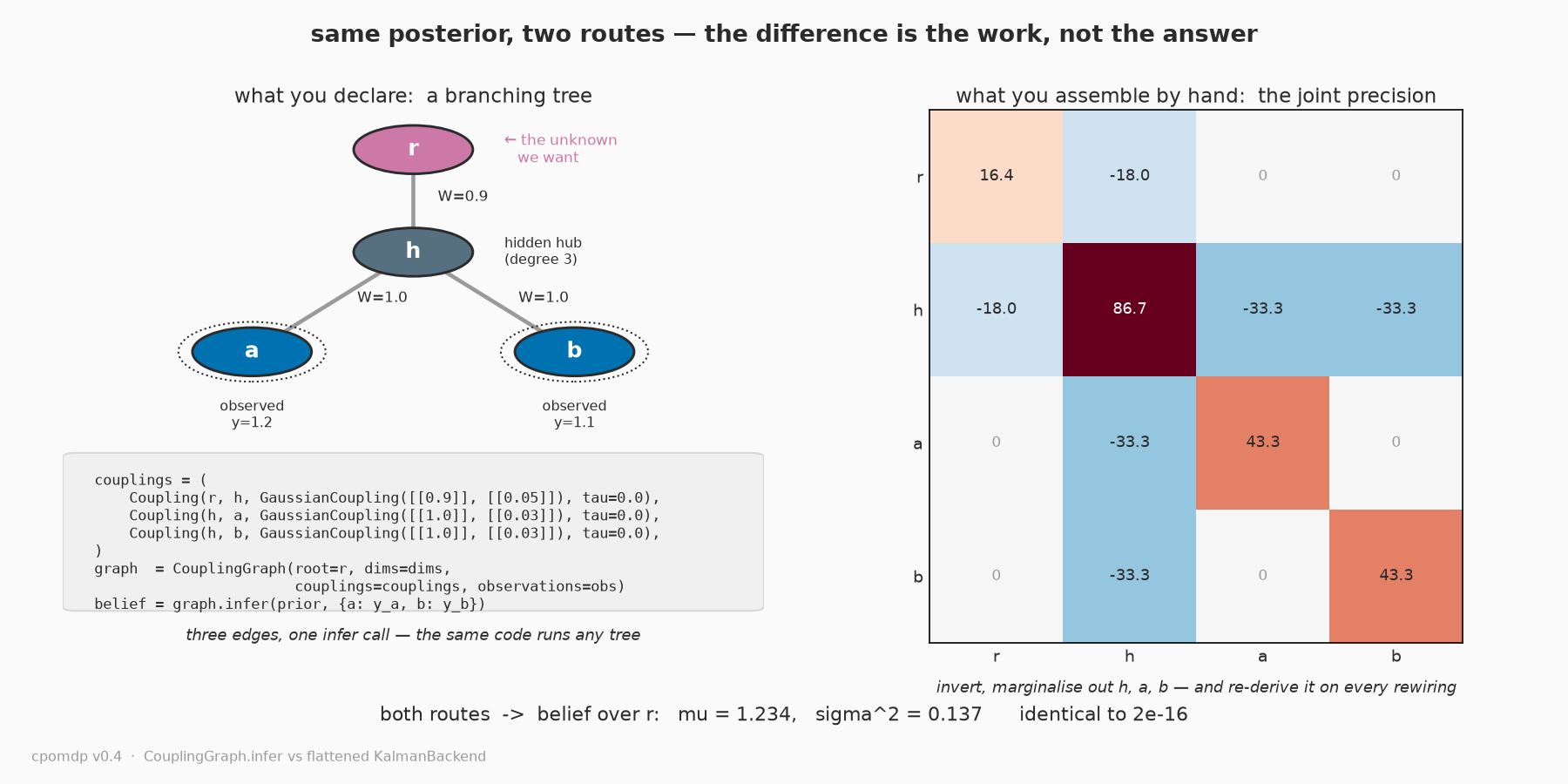
coupling_graph_figure.py --check prints both routes' root posteriors and their agreement,
no rendering.
A chemotaxis network, as its shape
chemotaxis_figure.py · v0.4 · ADR-012, ADR-020
The same declare-and-infer, on a real branching network instead of an abstract one. E. coli
chemotaxis is a receptor-driven CheA kinase hub feeding a fast CheY → motor branch and a slow
CheB methylation branch — a tree with a degree-3 node no chain can hold. cpomdp declares it as
a CouplingGraph and infers the hidden CheA hub from the downstream readouts (CheB and the two
motors), exact to a flattened Kalman.
It's the shape, not the biophysics: no CheB → receptor feedback (that's a loop, and a
CouplingGraph is a tree), no swimming, no efficiency. A faithful E. coli model is a
build-on-top, not a v0.4 feature (RFC-002, ADR-020). Reuses chemotaxis_model.py, the builder
the Phase-3 tests pin.
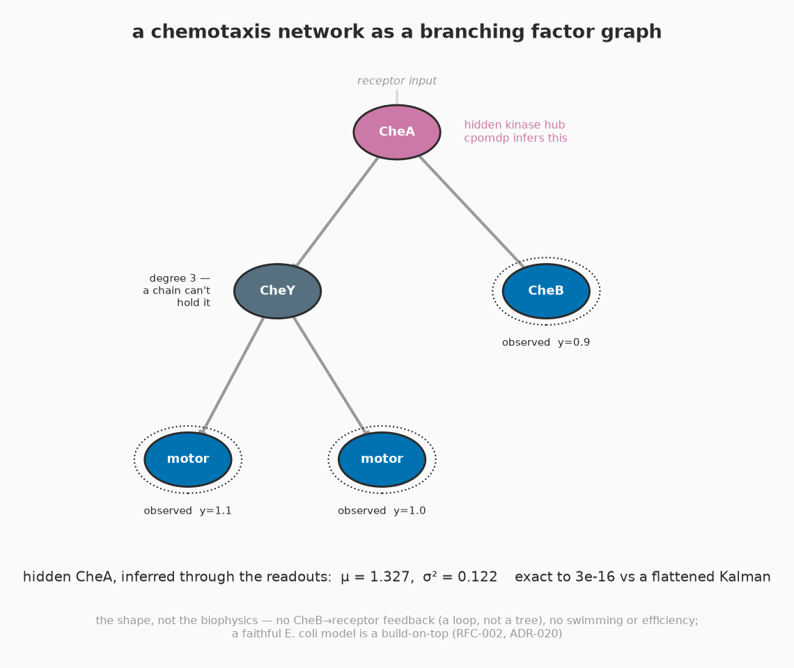
chemotaxis_figure.py --check prints the hidden-hub posterior from both routes and their
agreement.